1 Chapter 11: Why model?
This is the code for Chapter 11. Throughout this chapter and the rest of the book, we’ll use the tidyverse metapackage to load the core tidyverse packages, as well the broom package. In this chapter, the main packages we’ll be using are ggplot2 for data visualization, dplyr for data manipulation, and broom for tidying regression model results.
1.1 Program 11.1
To replicate Program 11.1, we first need to create the data set, binary_a_df.
library(tidyverse)
library(broom)

binary_a_df <- data.frame(
  a = c(rep(1, 8), rep(0, 8)),
  y = c(200, 150, 220, 110, 50, 180, 90, 170,
        170, 30, 70, 110, 80, 50, 10, 20)
)

ggplot(binary_a_df, aes(a, y)) +
  geom_point(size = 4, col = "white", fill = "#E69F00", shape = 21) +
  scale_x_continuous(breaks = c(0, 1), expand = expand_scale(.5)) +
  theme_minimal(base_size = 20)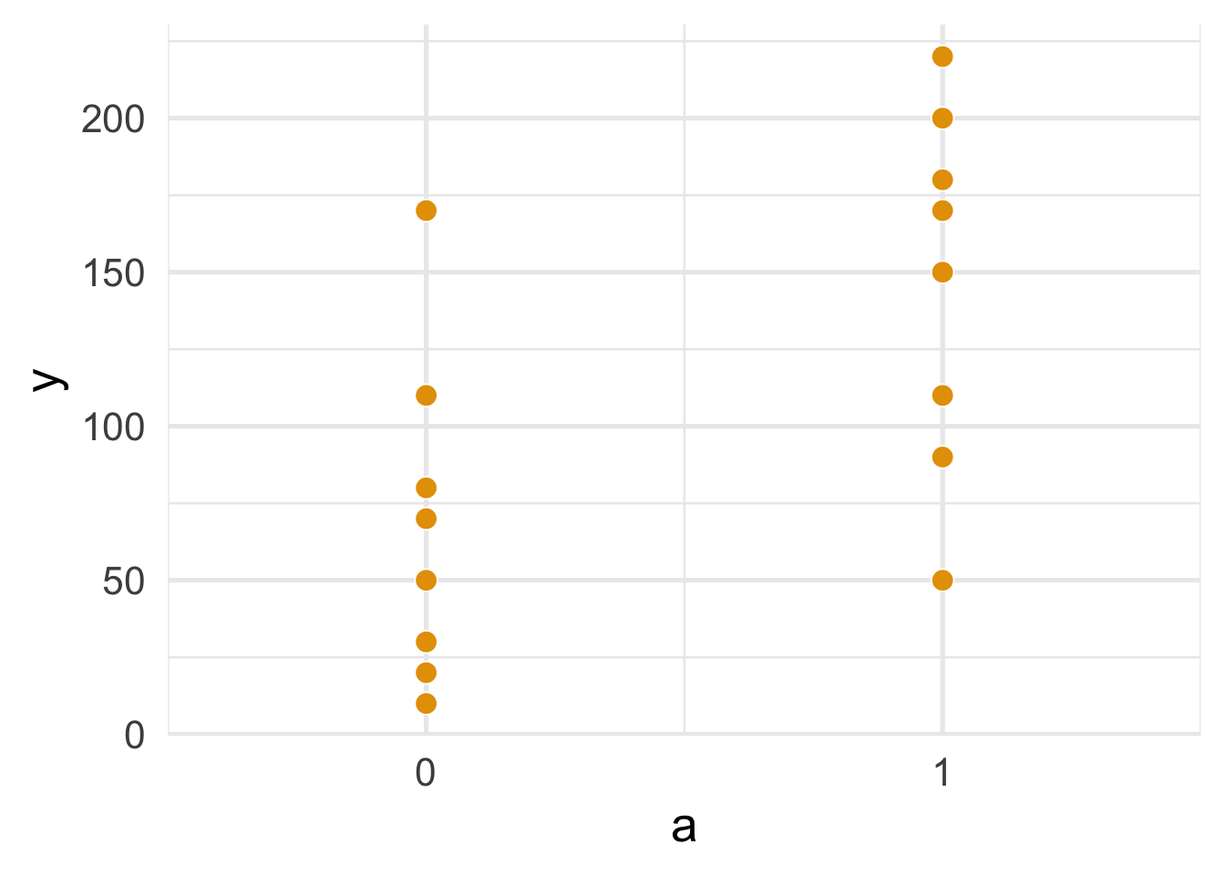
FIGURE 1.1: Figure 11.1
To summarize the data, we’ll use dplyr to group the dataset by a, then get the sample size, mean, standard deviation, and range. knitr::kable() is used to print the results nicely to a table. (For more information on the %>% pipe operator, see R for Data Science.)
binary_a_df %>%
  group_by(a) %>%
  summarize(
    n = n(),
    mean = mean(y),
    sd = sd(y),
    minimum = min(y),
    maximum = max(y)
  ) %>%
knitr::kable(digits = 2)| a | n | mean | sd | minimum | maximum |
|---|---|---|---|---|---|
| 0 | 8 | 67.50 | 53.12 | 10 | 170 |
| 1 | 8 | 146.25 | 58.29 | 50 | 220 |
Similarly, we’ll plot and summarize categorical_a_df.
categorical_a_df <- data.frame(a = sort(rep(1:4, 4)),
                               y = c(110, 80, 50, 40, 170, 30, 70, 50,
                                     110, 50, 180, 130, 200, 150, 220, 210))

ggplot(categorical_a_df, aes(a, y)) +
  geom_point(size = 4, col = "white", fill = "#E69F00",  shape = 21) +
  scale_x_continuous(breaks = 1:4, expand = expand_scale(.25)) +
  theme_minimal(base_size = 20)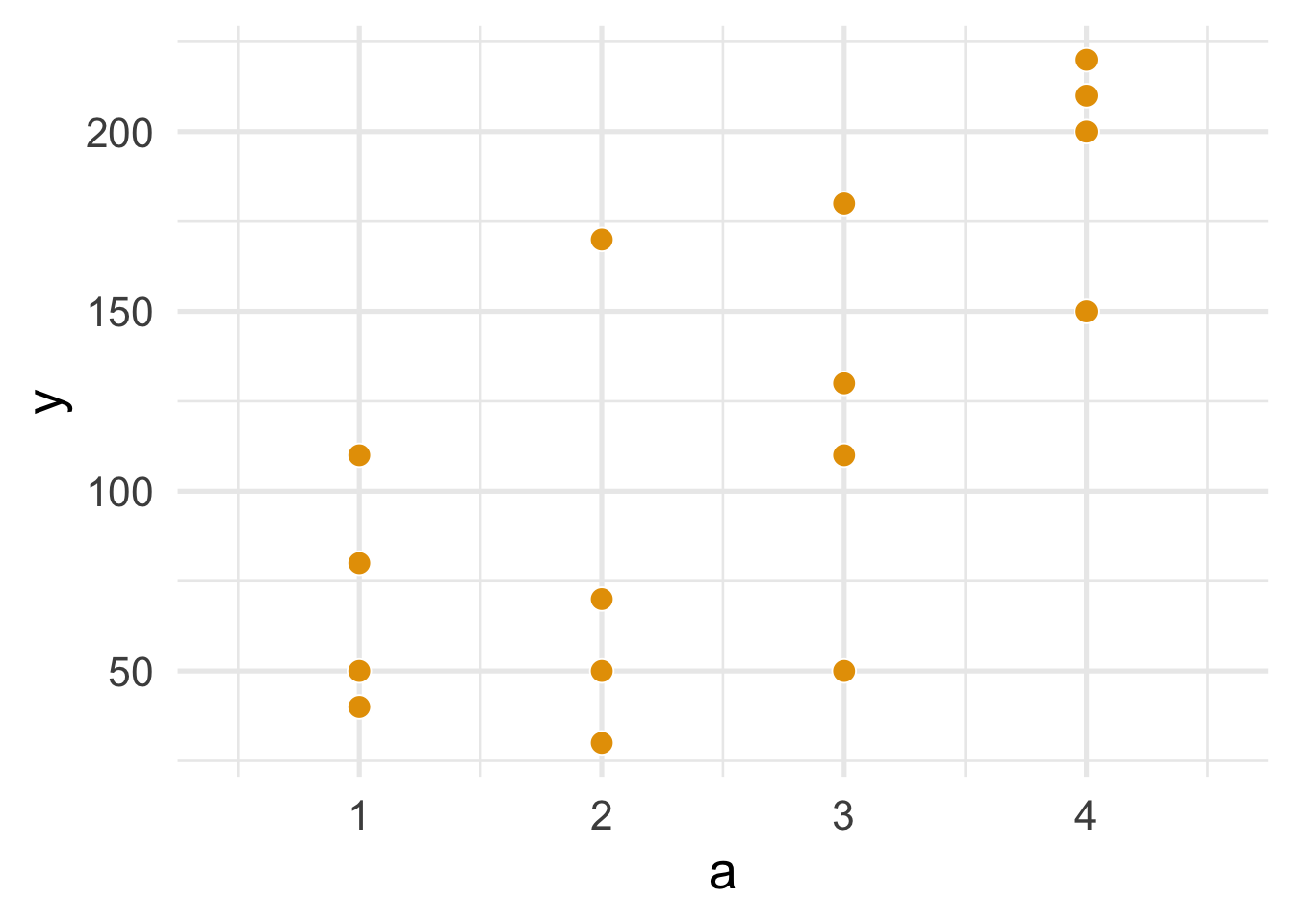
FIGURE 1.2: Figure 11.2
categorical_a_df %>%
  group_by(a) %>%
  summarize(
    n = n(),
    mean = mean(y),
    sd = sd(y),
    minimum = min(y),
    maximum = max(y)
  ) %>%
knitr::kable(digits = 2)| a | n | mean | sd | minimum | maximum |
|---|---|---|---|---|---|
| 1 | 4 | 70.0 | 31.62 | 40 | 110 |
| 2 | 4 | 80.0 | 62.18 | 30 | 170 |
| 3 | 4 | 117.5 | 53.77 | 50 | 180 |
| 4 | 4 | 195.0 | 31.09 | 150 | 220 |
1.2 Program 11.2
Program 11.2 uses a continuous exposure and outcome data, continuous_a_df. Plotting the points is similar to above.
continuous_a_df <- data.frame(
  a = c(3, 11, 17, 23, 29, 37, 41, 53,
        67, 79, 83, 97, 60, 71, 15, 45),
  y = c(21, 54, 33, 101, 85, 65, 157, 120,
        111, 200, 140, 220, 230, 217, 11, 190)
)

ggplot(continuous_a_df, aes(a, y)) +
  geom_point(size = 4, col = "white", fill = "#E69F00",  shape = 21) +
  theme_minimal(base_size = 20)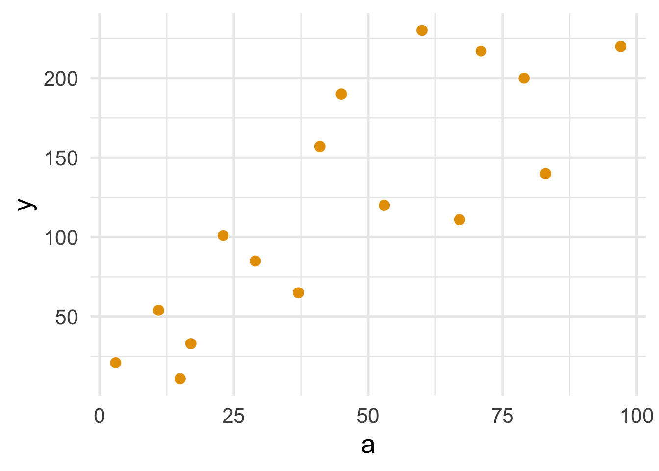
FIGURE 1.3: Figure 11.3
We’ll also add a regression line using geom_smooth() with method = "lm".
ggplot(continuous_a_df, aes(a, y)) +
  geom_point(size = 4, col = "white", fill = "grey85", shape = 21) +
  geom_smooth(method = "lm", se = FALSE, col = "#E69F00", size = 1.2) +
theme_minimal(base_size = 20) 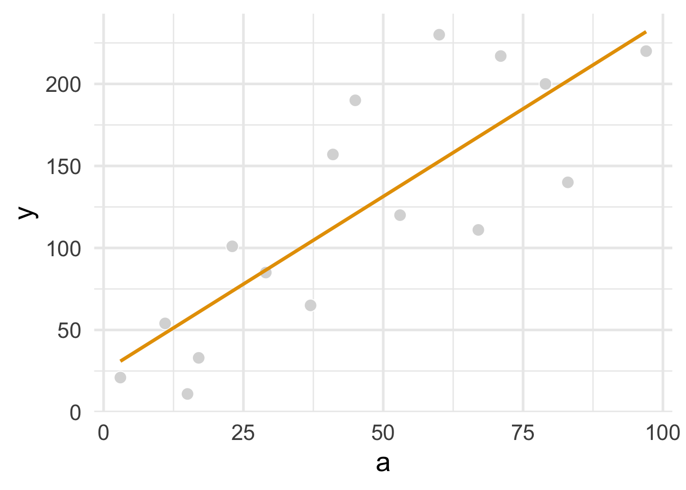
FIGURE 1.4: Figure 11.4
To fit an OLS regression model of a on y, we’ll uselm() and then tidy the results with tidy() from the broom package.
linear_regression <- lm(y ~ a, data = continuous_a_df)

linear_regression %>%
  # get the confidence intervals using `conf.int = TRUE`
  tidy(conf.int = TRUE) %>%
  # drop the test statistic and P-value
  select(-statistic, -p.value) %>%
knitr::kable(digits = 2)| term | estimate | std.error | conf.low | conf.high |
|---|---|---|---|---|
| (Intercept) | 24.55 | 21.33 | -21.20 | 70.29 |
| a | 2.14 | 0.40 | 1.28 | 2.99 |
To predict a value of y for when a = 90, we pass the linear regression model object linear_regression to the predict() function. We also give it a new data frame that contains only one value, a = 90.
linear_regression %>%
  predict(newdata = data.frame(a = 90))
## 1
## 216.89Similarly, using binary_a_df, which has a treatmant a that is a binary:
lm(y ~ a, data = binary_a_df) %>%
  tidy(conf.int = TRUE) %>%
  select(-statistic, -p.value) %>%
knitr::kable(digits = 2)| term | estimate | std.error | conf.low | conf.high |
|---|---|---|---|---|
| (Intercept) | 67.50 | 19.72 | 25.21 | 109.79 |
| a | 78.75 | 27.88 | 18.95 | 138.55 |
1.3 Program 11.3
Fitting and tidying a quadratic version of a is similar, but we use I() to include a^2.
smoothed_regression <- lm(y ~ a + I(a^2), data = continuous_a_df)

smoothed_regression %>%
  tidy(conf.int = TRUE) %>%
  select(-statistic, -p.value) %>%
  #  remove `I()` from the term name
  mutate(term = ifelse(term == "I(a^2)", "a^2", term)) %>%
knitr::kable(digits = 2) | term | estimate | std.error | conf.low | conf.high |
|---|---|---|---|---|
| (Intercept) | -7.41 | 31.75 | -75.99 | 61.18 |
| a | 4.11 | 1.53 | 0.80 | 7.41 |
| a^2 | -0.02 | 0.02 | -0.05 | 0.01 |
To plot the quadratic function, we give geom_smooth() a formula argument: formula = y ~ x + I(x^2).
ggplot(continuous_a_df, aes(a, y)) +
  geom_point(size = 4, col = "white", fill = "grey85", shape = 21) +
  geom_smooth(method = "lm", se = FALSE, col = "#E69F00", formula = y ~ x + I(x^2), size = 1.2) +
theme_minimal(base_size = 20) 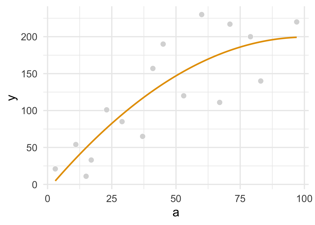
FIGURE 1.5: Figure 11.5
But predicting is done the same way.
smoothed_regression %>%
  predict(newdata = data.frame(a = 90))
## 1
## 197.1269